Survey-weighted Cox models.

Fit a proportional hazards model to data from a complex survey design.

svycoxph(formula, design,subset=NULL, rescale=TRUE, ...)
# S3 method for svycoxph
predict(object, newdata, se=FALSE,
    type=c("lp", "risk", "terms","curve"),...)
# S3 method for svycoxph
AIC(object, ..., k = 2)

Arguments

formula: Model formula. Any cluster() terms will be ignored.
design: survey.design object. Must contain all variables in the formula
subset: Expression to select a subpopulation
rescale: Rescale weights to improve numerical stability
object: A svycoxph object
newdata: New data for prediction
se: Compute standard errors? This takes a lot of memory for type="curve"
type: "curve" does predicted survival curves. The other values are passed to predict.coxph()
...: For AIC, more models to compare the AIC of. For svycoxph, other arguments passed to coxph.
k: The penalty per parameter that would be used under independent sampling: AIC has k=2

Details

The main difference between svycoxph function and the robust=TRUE option to coxph in the survival package is that this function accounts for the reduction in variance from stratified sampling and the increase in variance from having only a small number of clusters.

Note that strata terms in the model formula describe subsets that have a separate baseline hazard function and need not have anything to do with the stratification of the sampling.

The AIC method uses the same approach as AIC.svyglm, though the relevance of the criterion this optimises is a bit less clear than for generalised linear models.

The standard errors for predicted survival curves are available only by linearization, not by replicate weights (at the moment). Use withReplicates to get standard errors with replicate weights. Predicted survival curves are not available for stratified Cox models.

The standard errors use the delta-method approach of Williams (1995) for the Nelson-Aalen estimator, modified to handle the Cox model following Tsiatis (1981). The standard errors agree closely with survfit.coxph for independent sampling when the model fits well, but are larger when the model fits poorly. I believe the standard errors are equivalent to those of Lin (2000), but I don't know of any implementation that would allow a check.

Value

An object of class svycoxph for svycoxph, an object of class svykm or svykmlist for predict(,type="curve").

Warning

The standard error calculation for survival curves uses memory proportional to the sample size times the square of the number of events.

Author

Thomas Lumley

References

Binder DA. (1992) Fitting Cox's proportional hazards models from survey data. Biometrika 79: 139-147

Lin D-Y (2000) On fitting Cox's proportional hazards model to survey data. Biometrika 87: 37-47

Tsiatis AA (1981) A Large Sample Study of Cox's Regression Model. Annals of Statistics 9(1) 93-108

Williams RL (1995) "Product-Limit Survival Functions with Correlated Survival Times" Lifetime Data Analysis 1: 171--186

Examples

## Somewhat unrealistic example of nonresponse bias.
data(pbc, package="survival")

pbc$randomized<-with(pbc, !is.na(trt) & trt>0)
biasmodel<-glm(randomized~age*edema,data=pbc,family=binomial)
pbc$randprob<-fitted(biasmodel)
if (is.null(pbc$albumin)) pbc$albumin<-pbc$alb ##pre2.9.0

dpbc<-svydesign(id=~1, prob=~randprob, strata=~edema, data=subset(pbc,randomized))
rpbc<-as.svrepdesign(dpbc)

(model<-svycoxph(Surv(time,status>0)~log(bili)+protime+albumin,design=dpbc))
#> Call:
#> svycoxph(formula = Surv(time, status > 0) ~ log(bili) + protime + 
#>     albumin, design = dpbc)
#> 
#>               coef exp(coef) se(coef) robust se      z        p
#> log(bili)  0.88592   2.42522  0.09140   0.09048  9.791  < 2e-16
#> protime    0.24487   1.27745  0.07825   0.08122  3.015  0.00257
#> albumin   -1.04298   0.35240  0.21211   0.20454 -5.099 3.41e-07
#> 
#> Likelihood ratio test=  on 3 df, p=
#> n= 312, number of events= 144 

svycoxph(Surv(time,status>0)~log(bili)+protime+albumin,design=rpbc)
#> Call:
#> svycoxph.svyrep.design(formula = Surv(time, status > 0) ~ log(bili) + 
#>     protime + albumin, design = rpbc)
#> 
#>               coef exp(coef) se(coef)      z        p
#> log(bili)  0.88592   2.42522  0.09838  9.005  < 2e-16
#> protime    0.24487   1.27745  0.09373  2.612  0.00899
#> albumin   -1.04298   0.35240  0.21966 -4.748 2.05e-06
#> 
#> Likelihood ratio test=NA  on 3 df, p=NA
#> n= 312, number of events= 144 

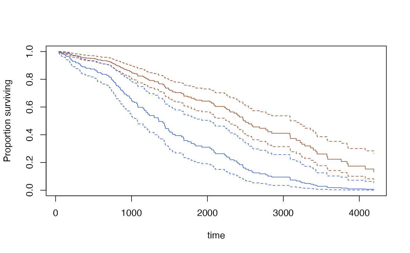
s<-predict(model,se=TRUE, type="curve",
     newdata=data.frame(bili=c(3,9), protime=c(10,10), albumin=c(3.5,3.5)))
plot(s[[1]],ci=TRUE,col="sienna")
lines(s[[2]], ci=TRUE,col="royalblue")

quantile(s[[1]], ci=TRUE)
#> 0.75  0.5 0.25 
#> 1435 2503 3574 
#> attr(,"ci")
#>      0.025 0.975
#> 0.75  1217  1786
#> 0.5   2256  3170
#> 0.25  3222   Inf
confint(s[[2]], parm=365*(1:5))
#>          0.025     0.975
#> 365  0.8375139 0.9453781
#> 730  0.7382750 0.8999016
#> 1095 0.4784105 0.7478460
#> 1460 0.3192009 0.6206764
#> 1825 0.2149475 0.5292978